Topic

Stanford CS229 Machine Learning

All digests tagged Stanford CS229 Machine Learning

Stanford CS229 Machine Learning | Spring 2026 | Lecture 20: GMM (EM), PCA thumbnail

· 1:18:56

Stanford CS229 Machine Learning | Spring 2026 | Lecture 20: GMM (EM), PCA

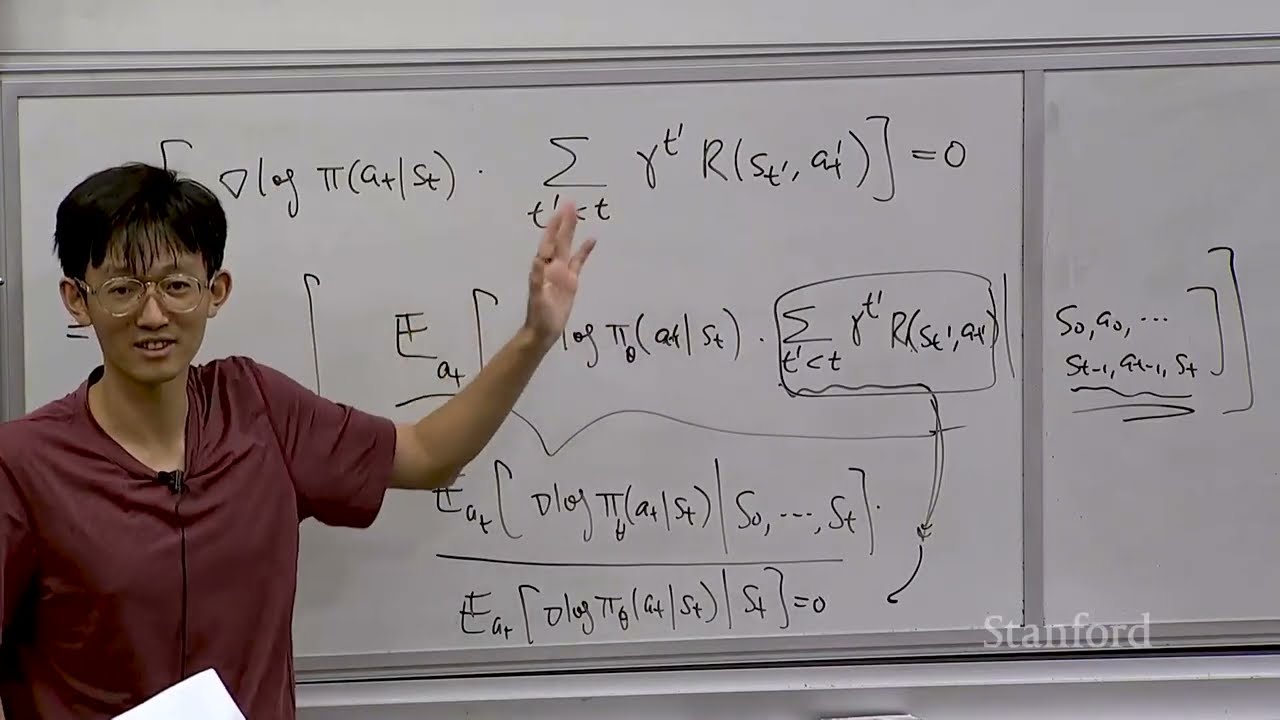
This lecture provides an advanced deep dive into training Large Language Models (LLMs) using Reinforcement Learning (RL). It reviews Policy Gradient methods, detailing the mathematical derivations and limitations. The core focus shifts to Proximal Policy Optimization (PPO), a critical algorithm for stabilizing RL updates by utilizing importance sampling ratios and clipping mechanisms. Finally, the lecture applies these concepts to LLM generation, explaining how Chain-of-Thought (CoT) prompting can be formalized as an MDP problem solved via PPO/SISO.

Key takeaways

  1. Policy Gradient Theory 20:40

    The policy gradient estimator is necessary because the dependency on parameters ($ heta$) is complex. The fundamental property that $ abla_{ heta} ext{E}_{ ext{P}_{ heta}}[ abla_{ heta} ext{log } ext{P}_{ heta}(a|s)]$ equals zero shows that without a reward function, there are no preferences to optimize for.

  2. Proximal Policy Optimization (PPO) 26:40

    PPO is designed to stabilize RL training by using importance sampling and clipping the objective function. This prevents the new policy ($ heta$) from deviating too far from the old policy ($ heta_{old}$), which helps maintain stable learning.

  3. LLM Generation as an MDP 1:01:40

    The LLM generation process is modeled as a Markov Decision Process (MDP). The state ($s_t$) includes the history, and the action ($a_t$) is the next generated token. The reward function is typically applied only at the end of the trajectory based on whether the final answer matches the ground truth.

  4. Chain-of-Thought (CoT) Training 1:05:00

    To train models for complex reasoning, RL can be used to reward the entire trajectory based on the final answer's correctness. This approach bypasses the need for explicit labeling of the internal 'thinking tokens,' focusing only on verifiable outcomes.

Watch on YouTube Full article

Stanford CS229 Machine Learning | Spring 2026 | Lecture 18: GMM (EM), PCA thumbnail

· 1:16:25

Stanford CS229 Machine Learning | Spring 2026 | Lecture 18: GMM (EM), PCA

This lecture provides a deep dive into Reinforcement Learning (RL), focusing on the formal framework of Markov Decision Processes (MDPs) and the Policy Gradient method. The core objective is to solve sequential decision-making problems by maximizing expected cumulative reward. Key concepts include defining states ($S$), actions ($A$), stochastic transition dynamics ($P(s'|s, a)$), and utilizing the Bellman equation for recursive value estimation. The lecture concludes with an explanation of the Policy Gradient algorithm (REINFORCE), detailing how to compute the gradient of the expected return using log-probability tricks, which is crucial for training policies in large models.

Key takeaways

  1. Sequential Decision Making & RL Fundamentals

    RL addresses sequential decision-making where actions have long-term ramifications. It requires balancing the trade-off between exploitation (using current best knowledge) and exploration (gathering information). Learning relies on maximizing a scalar reward signal rather than explicit labels or supervision.

  2. Markov Decision Process (MDP) Framework 4:00

    An MDP formally describes an environment using five components: State Set ($S$), Action Set ($A$), Transition Dynamics ($P(s'|s, a)$), Reward Function ($R$), and Discount Factor ($\gamma$). The Markov property ensures that the future state transition depends only on the current state and action, not on history.

  3. Value Functions and Bellman Equation 28:50

    The value function $V^{\pi}(s)$ estimates the expected total payoff starting at state $s$ under policy $\pi$. The optimal value, $V^*(s)$, is the maximum possible return. These values are solved recursively using the Bellman equation, which relates the current state's value to the expected discounted future rewards.

  4. Policy Gradient Method (REINFORCE) 43:20

    The Policy Gradient algorithm optimizes a stochastic policy $\pi_{\theta}(a|s)$ by maximizing the expected return $E[R]$. The gradient is computed using the log-probability trick, allowing the calculation of $\nabla_{\theta} E[R]$ through sampling, even when the dependency on $\theta$ only affects the sampling distribution.

Watch on YouTube Full article

Stanford CS229 Machine Learning | Spring 2026 | Lecture 16: Basic Concept in RL, Policy Gradient thumbnail

· 1:13:19

Stanford CS229 Machine Learning | Spring 2026 | Lecture 16: Basic Concept in RL, Policy Gradient

This lecture provides an advanced deep dive into optimizing Transformer architectures for efficiency and adapting Large Language Models (LLMs) for various downstream tasks. Key focus areas include reducing the quadratic complexity of attention through techniques like Grouped Query Attention (GQA) and Sliding Window Attention; scaling models using Mixture of Experts (MoE) to decouple memory from compute; and exploring prompt-based methods such as In-Context Learning, Few-Shot, and Zero-Shot learning for task adaptation without updating model parameters.

Key takeaways

  1. Efficiency in Attention Mechanisms 20:04

    The standard self-attention mechanism has $O(T^2)$ complexity (where T is sequence length). To mitigate this, techniques like Grouped Query Attention (GQA) reduce the number of keys and values used across heads by mapping multiple query groups to a smaller set of shared keys/values. Similarly, Sliding Window Attention limits attention to only recent history, reducing complexity to $O(T imes W)$ where W is the window size.

  2. Scaling with Mixture of Experts (MoE) 42:28

    MoE allows models to have a large total parameter count (e.g., 30B) while keeping the active computation small (e.g., 3B). This is achieved by using a routing module that directs an input vector to only a subset of specialized expert sub-networks, significantly improving compute efficiency.

  3. LLM Adaptation via Prompting 56:48

    For downstream tasks (e.g., sentiment analysis), models can be adapted using In-Context Learning (ICL). This involves concatenating task examples and the test input into the prompt sequence without updating model parameters, which is fundamentally different from traditional fine-tuning.

  4. Supervised Fine-Tuning (SFT) 1:04:00

    SFT involves collecting data in an instruction/answer pair format and training the model by minimizing the negative log likelihood of predicting the answer ($Y$) given the instruction ($X$). This is a supervised process that updates the model's weights.

Watch on YouTube Full article

Stanford CS229 Machine Learning | Spring 2026 | Lecture 14: Transformers, In-Context Learning thumbnail

· 1:17:32

Stanford CS229 Machine Learning | Spring 2026 | Lecture 14: Transformers, In-Context Learning

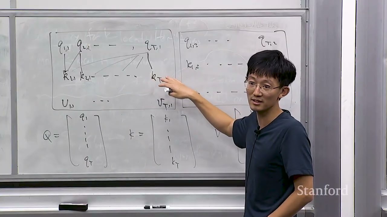
This lecture provides a deep technical dive into Large Language Models (LLMs), focusing on the Transformer architecture. Key concepts covered include subword tokenization (using techniques like Byte Pair Encoding - BPE) to convert text into numerical IDs, and modeling language distribution using auto-regressive conditional probabilities. The core mechanism is the self-attention layer, which uses Query (Q), Key (K), and Value (V) vectors to determine dependencies between tokens. A critical technical discussion centers on computational efficiency: standard attention has a quadratic $O(T^2)$ dependency on sequence length ($T$), leading to memory and computation bottlenecks for long contexts. Solutions like masking and specialized variants (e.g., Flash Attention) are discussed as methods to maintain performance while managing resource constraints.

Key takeaways

  1. Auto-Regressive Modeling 1:35

    LLMs model language distribution by decomposing the joint probability into a product of conditional probabilities: $P(X_t | X_{1...t-1})$. This requires generating tokens sequentially, making the process auto-regressive.

  2. Subword Tokenization (BPE) 3:30

    To handle rare or long words efficiently, models use subword tokenization (e.g., BPE), which breaks down text into smaller units (tokens). This allows leveraging common prefixes and suffixes to understand novel words.

  3. Self-Attention Mechanism 11:10

    The attention mechanism calculates the relevance between all tokens in a sequence using Query ($Q$), Key ($K$), and Value ($V$) vectors via an inner product: $ ext{Softmax}(Q K^T / ext{scale}) V$. The output is a weighted linear combination of $V$ vectors.

  4. Causal Masking for Auto-regression 21:20

    To ensure the model only predicts based on previous tokens (required for generation), a masking technique is applied to the attention matrix, setting all future dependencies to $- ext{infinity}$ before applying Softmax.

  5. Computational Bottleneck ($O(T^2)$) 30:00

    The standard self-attention mechanism has a computational and memory complexity that scales quadratically with sequence length $T$ (i.e., $O(T^2)$). This is the primary limitation for processing very long contexts.

Watch on YouTube Full article

Stanford CS229 Machine Learning | Spring 2026 | Lecture 12: Representation Learning thumbnail

· 1:15:57

Stanford CS229 Machine Learning | Spring 2026 | Lecture 12: Representation Learning

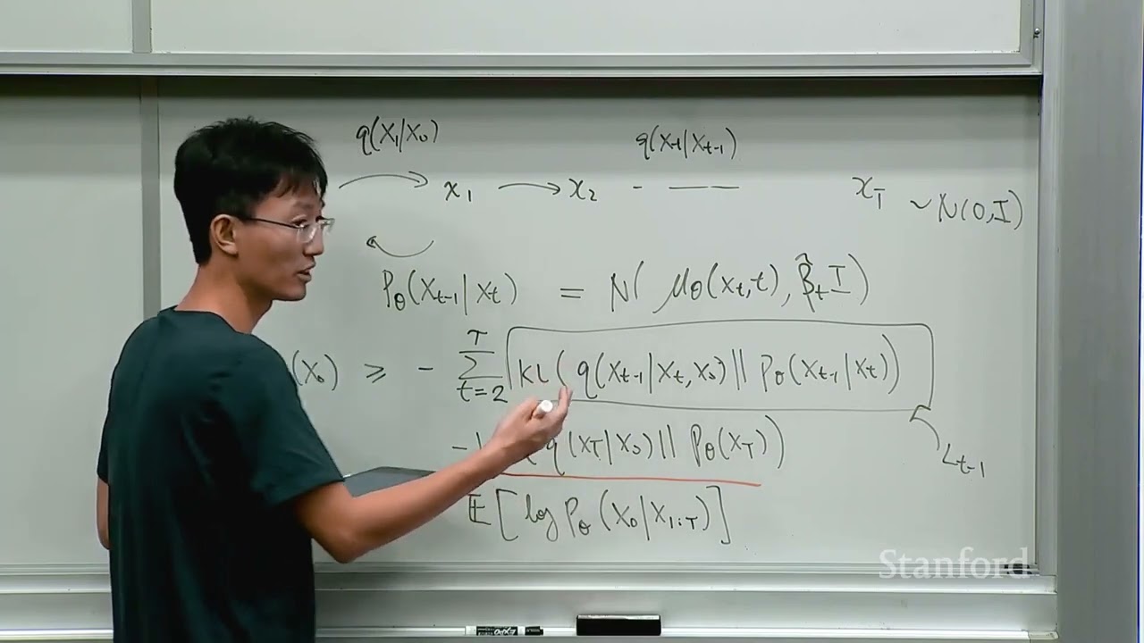
The lecture provides a deep dive into advanced generative and adaptation techniques, covering Diffusion Models, Foundation Model paradigms, and Representation Learning. Key technical focus areas include deriving the loss function for diffusion models by comparing true and predicted mean reconstructions ($\mu_{ ilde{t}, t}$ vs $\mu_{ heta, t}$). For large language models (LLMs), the discussion highlights the shift toward using massive unlabelled data for pre-training and adapting via zero-shot or few-shot methods. Finally, it details advanced parameter efficiency techniques like Linear Probing and Low-Rank Adaptation (LoRA), which are crucial for managing memory and compute when deploying large models across multiple users.

Key takeaways

  1. Diffusion Model Training Objective 33:55

    The training objective is derived from the lower bound on $\log p_ heta(x_0)$, simplifying to minimizing a sum of terms ($\mathcal{L}_{t-1}$) that compares the mean predicted reconstruction ($\mu_{ heta, t}$) with the true process mean ($\mu_{ ilde{t}, t}$). This loss function is used to train the model to predict noise/reconstruct missing information at each time step.

  2. Foundation Model Paradigm Shift 1:02:00

    Modern LLMs utilize a paradigm shift involving pre-training on massive unlabelled data and adapting via zero-shot or few-shot learning, reducing the need for collecting extensive downstream labeled datasets. The goal is to build a general foundation that can be adapted to unlimited tasks.

  3. Low-Rank Adaptation (LoRA) Efficiency 1:15:00

    To adapt massive pre-trained models without changing all parameters ($\theta$), LoRA restricts the weight update matrix $\Delta W$ to a low rank ($A B$). This significantly reduces the number of trainable parameters and is critical for memory efficiency, especially when serving multiple users.

Watch on YouTube Full article

Stanford CS229 Machine Learning | Spring 2026 | Lecture 11: Diffusion Models thumbnail

· 1:22:31

Stanford CS229 Machine Learning | Spring 2026 | Lecture 11: Diffusion Models

The lecture introduces Diffusion Models as a predominant class of generative models used for tasks like image, video, and action generation. The core mechanism involves two processes: the forward process (gradually adding Gaussian noise to an original clean image $X_0$ over time steps $T$) and the reverse process (learning to iteratively denoise the noisy data back to a clean state). Training these models is achieved by applying the Evidence Lower Bound (ELBO) framework, which minimizes the Kullback-Leibler (KL) divergence between the true conditional distribution and the parameterized model's prediction.

Key takeaways

  1. Diffusion Models Overview

    These models are generative frameworks that can be applied to images, videos, and robotics actions. They are noted as a superior approach compared to GANs and Variational Autoencoders (VAEs) for image generation.

  2. Forward vs. Reverse Process 4:05

    The forward process is a fixed, known noising process that transforms $X_0$ to noise $X_T$. The reverse process is the learned component, parameterized by $ heta$, which predicts $p_ heta(X_{t-1}|X_t)$—the step-by-step denoising path.

  3. Training Objective (ELBO) 6:25

    The goal is to maximize the marginal likelihood $ ext{log } p_ heta(X_0)$ by applying the Evidence Lower Bound (ELBO). This involves minimizing the KL divergence between the true posterior $q(X_{t-1}|X_t, X_0)$ and the parameterized model's distribution.

Watch on YouTube Full article

Stanford CS229 Machine Learning | Spring 2026 | Lecture 8: Neural Networks 2 (Backprop) thumbnail

· 1:02:13

Stanford CS229 Machine Learning | Spring 2026 | Lecture 8: Neural Networks 2 (Backprop)

This lecture provides a deep theoretical dive into Backpropagation and Automatic Differentiation, establishing it as an efficient method for computing gradients in complex neural networks. The core principle is that any differentiable network can be viewed as a 'differentiable circuit' or computational graph. This allows the gradient (the backward pass) to be computed with a time complexity proportional to the number of parameters ($O(N)$), matching the efficiency of the forward pass, regardless of how complex the underlying function is.

Key takeaways

  1. Automatic Differentiation and Computational Graphs 2:00

    The gradient computation (backward pass) can be viewed as traversing a differentiable circuit. This method allows for efficient calculation because it reuses intermediate results, unlike expanding the function into a traditional mathematical formula.

  2. Efficiency of Gradient Computation 2:40

    The fundamental theorem states that if a differentiable circuit of size $N$ computes a real-valued function, its gradient can also be computed in time complexity $O(N)$. This means the forward pass (evaluating loss) and the backward pass (calculating gradients) have similar computational costs.

  3. Chain Rule Application for Backprop 5:50

    Backpropagation is an application of the Chain Rule. By knowing the gradient with respect to an intermediate variable ($U$), one can compute the gradient with respect to its input ($Z$) using matrix multiplication involving the Jacobian (or transpose of the Jacobian). This process allows computation to proceed layer by layer.

Watch on YouTube Full article

Stanford CS229 Machine Learning | Spring 2026 | Lecture 6: Dataset Split, ML Advice thumbnail

· 1:18:27

Stanford CS229 Machine Learning | Spring 2026 | Lecture 6: Dataset Split, ML Advice

This lecture provides a deep dive into the fundamental challenge of machine learning: generalization. It systematically analyzes how models trained on finite, noisy samples can be selected to perform reliably on unseen data. Key concepts include decomposing test error into bias (model class limitation), variance (sensitivity to training data), and noise (measurement error). The discussion covers classical techniques like regularization (e.g., Ridge Regression) for reducing variance at the cost of slight bias, modern phenomena like Double Descent in overparameterized models, and practical model selection methods such as K-fold cross validation and Hyperband.

Key takeaways

  1. Bias-Variance Decomposition 20:05

    Test error is decomposed into three components: noise (intrinsic data error), squared bias (how far the average prediction is from the true function, dependent on model class), and variance (how much the prediction jumps around across different training sets). Minimizing test error requires balancing these three sources of error.

  2. Regularization as Variance Reduction 30:05

    Regularization techniques, such as adding an $L_2$ penalty (Ridge Regression), constrain the model weights ($ heta$) to prevent them from becoming too large. This stabilizes the model, significantly reducing variance while accepting a small increase in bias.

  3. Modern ML Phenomena: Double Descent 1:03:25

    The classical Bias-Variance curve suggests that test error must rise after a certain model complexity threshold. However, modern models can exhibit 'Double Descent,' where the test error decreases again in the massively overparameterized regime (i.e., having more parameters than data points).

  4. Model Selection and Hyperparameter Tuning 50:50

    To prevent information leakage from the test set, techniques like K-fold cross validation are used. For compute efficiency in tuning hyperparameters (e.g., regularization strength $ ho$), algorithms like Hyperband efficiently allocate computational resources to promising model configurations.

Watch on YouTube Full article

Stanford CS229 Machine Learning | Spring 2026 | Lecture 4: Exponential Family, GLMs classification thumbnail

· 1:14:12

Stanford CS229 Machine Learning | Spring 2026 | Lecture 4: Exponential Family, GLMs classification

The lecture introduces the Exponential Family as a unifying framework for numerous statistical models, including linear regression, logistic regression, Gaussian error modeling, and multinomial classification (Softmax). By showing that these diverse distributions share a common mathematical form, the theory demonstrates that core machine learning procedures—such as inference (calculating expected values) and parameter estimation (learning)—can be generalized across all members of this family. This foundational understanding is critical for modern AI architectures, particularly those utilizing Softmax in large language models.

Key takeaways

  1. The Exponential Family Unification 2:00

    Many common distributions (Bernoulli, Gaussian, Multinomial) can be written into a single functional form. This allows for the generalization of model building and analysis across different data types.

  2. Inference and Learning are Generalized 3:30

    The structure of the exponential family ensures that key statistical operations, such as computing the expected value (inference) and performing maximum likelihood estimation (learning), follow a consistent mathematical pattern regardless of the specific distribution used.

  3. Softmax in Multiclass Classification 6:10

    The Softmax function is presented as the standard mechanism for multiclass classification, allowing prediction over $K$ discrete values. Mathematically, it fits within the exponential family structure and generalizes logistic regression (the two-class case).

  4. Generalized Linear Models (GLMs) 10:50

    The GLM framework ties the abstract error models to practical supervised learning. The model predicts a distribution over $Y$ given features $X$, and the loss function is derived directly from maximizing the log-likelihood of this distribution.

Watch on YouTube Full article