Topic

Markov Decision Processes (MDP)

All digests tagged Markov Decision Processes (MDP)

Stanford AA203 Optimal and Learning-Based Control | Spring 2026 | Lecture 9: Stochastic Dyn. Program thumbnail

· 1:17:01

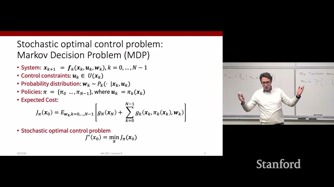
Stanford AA203 Optimal and Learning-Based Control | Spring 2026 | Lecture 9: Stochastic Dyn. Program

This lecture details the extension of optimal control theory from deterministic settings to stochastic environments using Markov Decision Processes (MDPs). The core methodology involves defining state transitions and costs that incorporate random disturbances ($w_k$). For finite-horizon problems, the solution relies on adapting the Bellman recursion by taking the expectation over all disturbance realizations. Crucially, for infinite-horizon MDPs—which are foundational to Reinforcement Learning (RL)—the problem is simplified by assuming stationarity and introducing a discount factor ($\gamma$), leading to fixed-point equations for the optimal value function ($V^*$) and the Q-function ($Q^*$).

Key takeaways

  1. Stochastic State Dynamics (MDP) 2:00

    The state update is modeled as $x_{k+1} = f(x_k, u_k, w_k)$, where $w_k$ is a random disturbance. The system must adhere to the Markovian assumption: the probability distribution of $w_k$ can only depend on the current state ($x_k$) and control ($u_k$), not on the history of previous states or disturbances.

  2. Finite-Horizon Optimization 4:00

    The notion of optimality is defined by minimizing the expected cost, $\mathbb{E}[ ext{Cost}]$, over all possible disturbance realizations. The solution uses a backward dynamic programming recursion (Bellman equation) to find the optimal closed-loop policy $\pi^*$.

  3. Infinite-Horizon MDPs and Discounting 10:20

    To solve problems over an infinite number of stages, a discount factor ($\gamma \in [0, 1]$) is introduced to ensure the convergence of the expected cumulative reward. The optimal value function $V^*$ satisfies a fixed-point equation: $V^*(x) = \max_{u} \{ R(x, u) + \gamma \mathbb{E}[V^*(x')]\}$.

  4. The Q-Function Formulation 17:30

    For computational tractability in learning settings where the transition kernel is unknown, the problem can be reformulated using the Q-function ($Q^*$), which represents the expected cumulative reward starting at state $x$ and taking action $u$, followed by optimal actions: $Q^*(x, u) = R(x, u) + \gamma \sum_{x'} T(x'|x, u) V^*(x')$.

Watch on YouTube Full article

Stanford CS229 Machine Learning | Spring 2026 | Lecture 18: GMM (EM), PCA thumbnail

· 1:16:25

Stanford CS229 Machine Learning | Spring 2026 | Lecture 18: GMM (EM), PCA

This lecture provides a deep dive into Reinforcement Learning (RL), focusing on the formal framework of Markov Decision Processes (MDPs) and the Policy Gradient method. The core objective is to solve sequential decision-making problems by maximizing expected cumulative reward. Key concepts include defining states ($S$), actions ($A$), stochastic transition dynamics ($P(s'|s, a)$), and utilizing the Bellman equation for recursive value estimation. The lecture concludes with an explanation of the Policy Gradient algorithm (REINFORCE), detailing how to compute the gradient of the expected return using log-probability tricks, which is crucial for training policies in large models.

Key takeaways

  1. Sequential Decision Making & RL Fundamentals

    RL addresses sequential decision-making where actions have long-term ramifications. It requires balancing the trade-off between exploitation (using current best knowledge) and exploration (gathering information). Learning relies on maximizing a scalar reward signal rather than explicit labels or supervision.

  2. Markov Decision Process (MDP) Framework 4:00

    An MDP formally describes an environment using five components: State Set ($S$), Action Set ($A$), Transition Dynamics ($P(s'|s, a)$), Reward Function ($R$), and Discount Factor ($\gamma$). The Markov property ensures that the future state transition depends only on the current state and action, not on history.

  3. Value Functions and Bellman Equation 28:50

    The value function $V^{\pi}(s)$ estimates the expected total payoff starting at state $s$ under policy $\pi$. The optimal value, $V^*(s)$, is the maximum possible return. These values are solved recursively using the Bellman equation, which relates the current state's value to the expected discounted future rewards.

  4. Policy Gradient Method (REINFORCE) 43:20

    The Policy Gradient algorithm optimizes a stochastic policy $\pi_{\theta}(a|s)$ by maximizing the expected return $E[R]$. The gradient is computed using the log-probability trick, allowing the calculation of $\nabla_{\theta} E[R]$ through sampling, even when the dependency on $\theta$ only affects the sampling distribution.

Watch on YouTube Full article