Stanford AA203 Optimal and Learning-Based Control | Spring 2026 | Lecture 9: Stochastic Dyn. Program
Summary
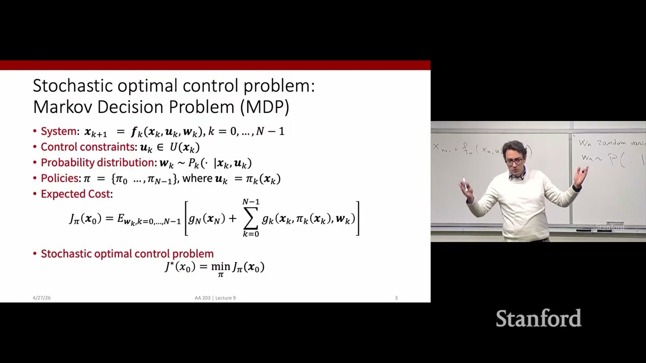
This lecture details the extension of optimal control theory from deterministic settings to stochastic environments using Markov Decision Processes (MDPs). The core methodology involves defining state transitions and costs that incorporate random disturbances ($w_k$). For finite-horizon problems, the solution relies on adapting the Bellman recursion by taking the expectation over all disturbance realizations. Crucially, for infinite-horizon MDPs—which are foundational to Reinforcement Learning (RL)—the problem is simplified by assuming stationarity and introducing a discount factor ($\gamma$), leading to fixed-point equations for the optimal value function ($V^*$) and the Q-function ($Q^*$).
Key takeaways
-
Stochastic State Dynamics (MDP)
2:00
The state update is modeled as $x_{k+1} = f(x_k, u_k, w_k)$, where $w_k$ is a random disturbance. The system must adhere to the Markovian assumption: the probability distribution of $w_k$ can only depend on the current state ($x_k$) and control ($u_k$), not on the history of previous states or disturbances.
-
Finite-Horizon Optimization
4:00
The notion of optimality is defined by minimizing the expected cost, $\mathbb{E}[ ext{Cost}]$, over all possible disturbance realizations. The solution uses a backward dynamic programming recursion (Bellman equation) to find the optimal closed-loop policy $\pi^*$.
-
Infinite-Horizon MDPs and Discounting
10:20
To solve problems over an infinite number of stages, a discount factor ($\gamma \in [0, 1]$) is introduced to ensure the convergence of the expected cumulative reward. The optimal value function $V^*$ satisfies a fixed-point equation: $V^*(x) = \max_{u} \{ R(x, u) + \gamma \mathbb{E}[V^*(x')]\}$.
-
The Q-Function Formulation
17:30
For computational tractability in learning settings where the transition kernel is unknown, the problem can be reformulated using the Q-function ($Q^*$), which represents the expected cumulative reward starting at state $x$ and taking action $u$, followed by optimal actions: $Q^*(x, u) = R(x, u) + \gamma \sum_{x'} T(x'|x, u) V^*(x')$.
Technical details
-
Stochastic Dynamics and Assumptions
90s
The state transition is defined by $x_{k+1} = f(x_k, u_k, w_k)$. The key assumption is that the disturbance $w_k$ must be Markovian, meaning its distribution depends only on $(x_k, u_k)$ and not on the process history.
-
Bellman Recursion (Finite Horizon)
320s
The optimal cost-to-go $J_{k+1}(x_{k+1})$ is found recursively by minimizing the expected value of the sum of current and future costs: $\min_{u_k} \mathbb{E}[C(x_k, u_k, w_k) + J_{k+1}(x_{k+1})]$.
-
Stochastic LQR Adaptation
800s
For Linear Quadratic Regulator (LQR) problems with stochastic dynamics ($w$ is Gaussian, zero mean, covariance $\Sigma$), the optimal control policy remains linear feedback. The expectation of the quadratic cost term involving $w$ simplifies using the property: $\mathbb{E}[w^T P_{k+1} w] = \text{Trace}(P_{k+1} \Sigma)$.
-
Optimal Action Selection (Learning Context)
1250s
If the optimal Q-function $Q^*(x, u)$ is known (e.g., via an oracle), the optimal action $u^*$ can be found by solving a simple maximization problem: $u^* = \arg\max_{u} Q^*(x, u)$.
Mentioned resources
Channel & topics
Watch on YouTube · Back to latest
This independent, AI-assisted summary is provided for commentary and informational purposes. It may contain errors or omit important context. Please watch the original video for the creator's complete presentation. Video, thumbnail, and related copyrights belong to their respective owners.