Topic

Optimal Control Theory

All digests tagged Optimal Control Theory

Stanford AA203 Optimal and Learning-Based Control | Spring 2026 | Lecture 19: Model-Based RL thumbnail

· 1:21:50

Stanford AA203 Optimal and Learning-Based Control | Spring 2026 | Lecture 19: Model-Based RL

This lecture reviews advanced topics in Reinforcement Learning (RL), transitioning from model-free policy optimization methods (TRPO/PPO) to the critical challenges of Model-Based RL. The core focus is addressing model uncertainty when using learned dynamics for planning. Techniques such as Bayesian statistics, Gaussian Processes (GPs), and Ensembles are introduced to quantify epistemic uncertainty, allowing planners to compute expected rewards by averaging predictions over a posterior distribution of possible models.

Key takeaways

  1. PPO/TRPO for Policy Optimization 16:15

    Policy optimization methods (like TRPO and PPO) define a surrogate objective function to estimate the policy gradient, enabling continuous updates. PPO uses a clipped ratio ($ ext{clip}(r_{ heta}, 1- ext{eps}, 1+ ext{eps})$) to constrain the new policy's divergence from the old one, stabilizing training without requiring complex second-order optimization.

  2. Model-Based RL Limitations 25:00

    The basic model-based recipe (collect data $ ightarrow$ fit dynamics $P(s'|s, a)$ $ ightarrow$ plan) fails when dealing with complex or nonlinear dynamics because extrapolation outside the observed state distribution is unreliable. This issue of generalization and distribution shift must be addressed.

  3. Quantifying Model Uncertainty 35:00

    To improve model-based planning, uncertainty quantification is necessary. The distinction between Aleatoric (inherent noise) and Epistemic (model uncertainty) is crucial. Bayesian approaches treat this by modeling the posterior distribution over parameters ($ heta$), allowing for prediction averaging across all plausible models.

  4. Ensemble Methods for Uncertainty 46:40

    A practical approach to estimate model uncertainty is using ensembles: training multiple independent neural network copies. The average of their predictions approximates the predictive posterior distribution, effectively exploring multimodal solution landscapes without requiring complex analytical derivations.
Watch on YouTube Full article

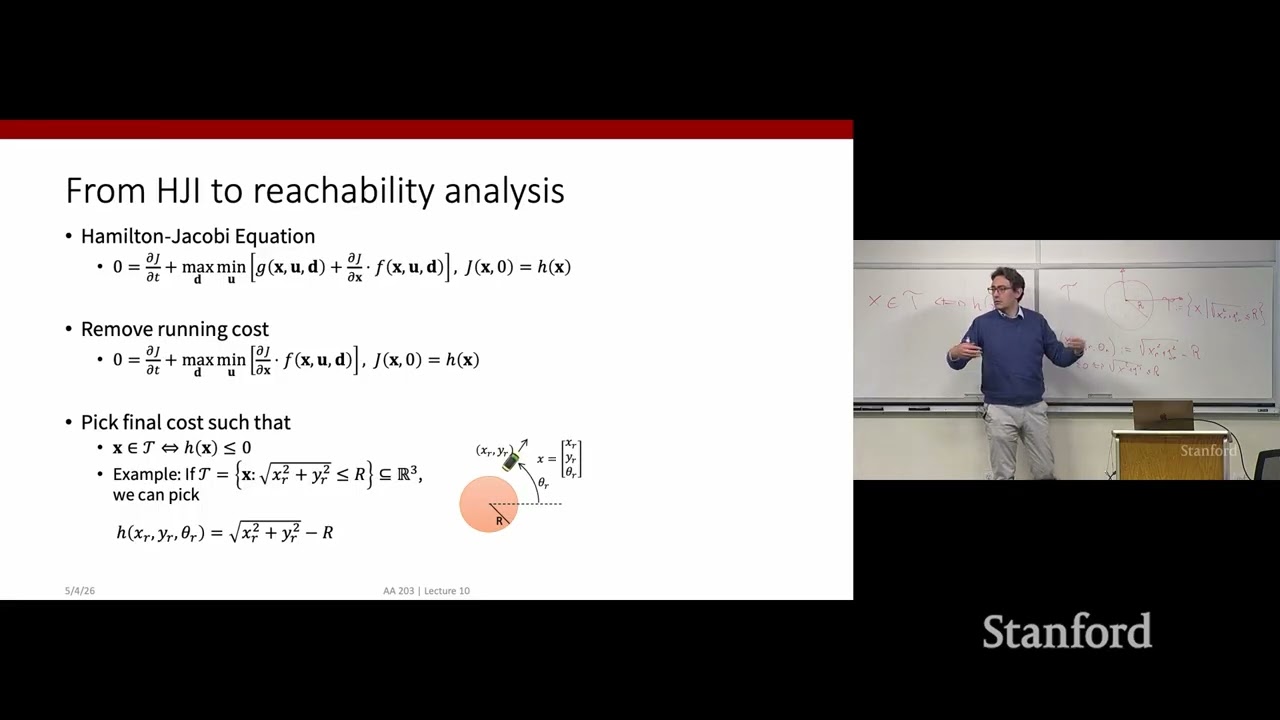
Stanford AA203 Optimal and Learning-Based Control | Spring 2026 | Lecture 11: Introduction to MPC thumbnail

· 1:13:36

Stanford AA203 Optimal and Learning-Based Control | Spring 2026 | Lecture 11: Introduction to MPC

This lecture provides a deep dive into advanced control theory, transitioning from theoretical concepts like Hamilton-Jacobi-Isaacs (HJI) equations for computing reachable sets to the practical framework of Model Predictive Control (MPC). The discussion emphasizes that MPC achieves closed-loop performance by repeatedly solving an open-loop optimal control problem over a finite horizon (receding horizon optimization). Key theoretical challenges addressed include ensuring persistent feasibility and stability, which requires leveraging concepts from invariant set theory.

Key takeaways

  1. Reachable Sets via HJI Equation 0:35

    Avoidance sets and reachable sets are computed by solving a differential game using the Hamilton-Jacobi-Isaacs (HJI) equation. This involves reframing the Boolean problem of set membership into an optimal control cost function $h(x)$ [0:35].

  2. Backward Reachable Tube (BRT) 7:40

    To ensure safety over the entire trajectory, not just the endpoint, one must compute a Backward Reachable Tube (BRT). This is achieved by modifying the cost function to minimize the minimum value of $h(x)$ across the entire optimization horizon [7:40].

  3. MPC Receding Horizon Principle 19:30

    MPC solves an open-loop optimal control problem over a finite prediction horizon $[t, t+N_p]$ at each time step $t$. It then uses only the first computed input ($u_t$) and discards the rest of the plan, recomputing everything from scratch based on new state measurements (receding horizon) [19:30].

  4. MPC Design Goals 36:00

    The primary goals when designing an MPC controller are ensuring persistent feasibility (the problem remains solvable at all future times) and guaranteeing stability (convergence to the desired state, e.g., the origin) [36:00].

  5. Invariant Sets for Feasibility 1:08:40

    To guarantee persistent feasibility in MPC, one must identify a control invariant set $\mathcal{C}$. This is a set where, if the system starts within it, there exists a control input $u$ that guarantees the next state remains inside $\mathcal{C}$ [38:00].

Watch on YouTube Full article

Stanford CS229 Machine Learning | Spring 2026 | Lecture 18: GMM (EM), PCA thumbnail

· 1:16:25

Stanford CS229 Machine Learning | Spring 2026 | Lecture 18: GMM (EM), PCA

This lecture provides a deep dive into Reinforcement Learning (RL), focusing on the formal framework of Markov Decision Processes (MDPs) and the Policy Gradient method. The core objective is to solve sequential decision-making problems by maximizing expected cumulative reward. Key concepts include defining states ($S$), actions ($A$), stochastic transition dynamics ($P(s'|s, a)$), and utilizing the Bellman equation for recursive value estimation. The lecture concludes with an explanation of the Policy Gradient algorithm (REINFORCE), detailing how to compute the gradient of the expected return using log-probability tricks, which is crucial for training policies in large models.

Key takeaways

  1. Sequential Decision Making & RL Fundamentals

    RL addresses sequential decision-making where actions have long-term ramifications. It requires balancing the trade-off between exploitation (using current best knowledge) and exploration (gathering information). Learning relies on maximizing a scalar reward signal rather than explicit labels or supervision.

  2. Markov Decision Process (MDP) Framework 4:00

    An MDP formally describes an environment using five components: State Set ($S$), Action Set ($A$), Transition Dynamics ($P(s'|s, a)$), Reward Function ($R$), and Discount Factor ($\gamma$). The Markov property ensures that the future state transition depends only on the current state and action, not on history.

  3. Value Functions and Bellman Equation 28:50

    The value function $V^{\pi}(s)$ estimates the expected total payoff starting at state $s$ under policy $\pi$. The optimal value, $V^*(s)$, is the maximum possible return. These values are solved recursively using the Bellman equation, which relates the current state's value to the expected discounted future rewards.

  4. Policy Gradient Method (REINFORCE) 43:20

    The Policy Gradient algorithm optimizes a stochastic policy $\pi_{\theta}(a|s)$ by maximizing the expected return $E[R]$. The gradient is computed using the log-probability trick, allowing the calculation of $\nabla_{\theta} E[R]$ through sampling, even when the dependency on $\theta$ only affects the sampling distribution.

Watch on YouTube Full article