Stanford AA203 Optimal and Learning-Based Control | Spring 2026 | Lecture 11: Introduction to MPC
Summary
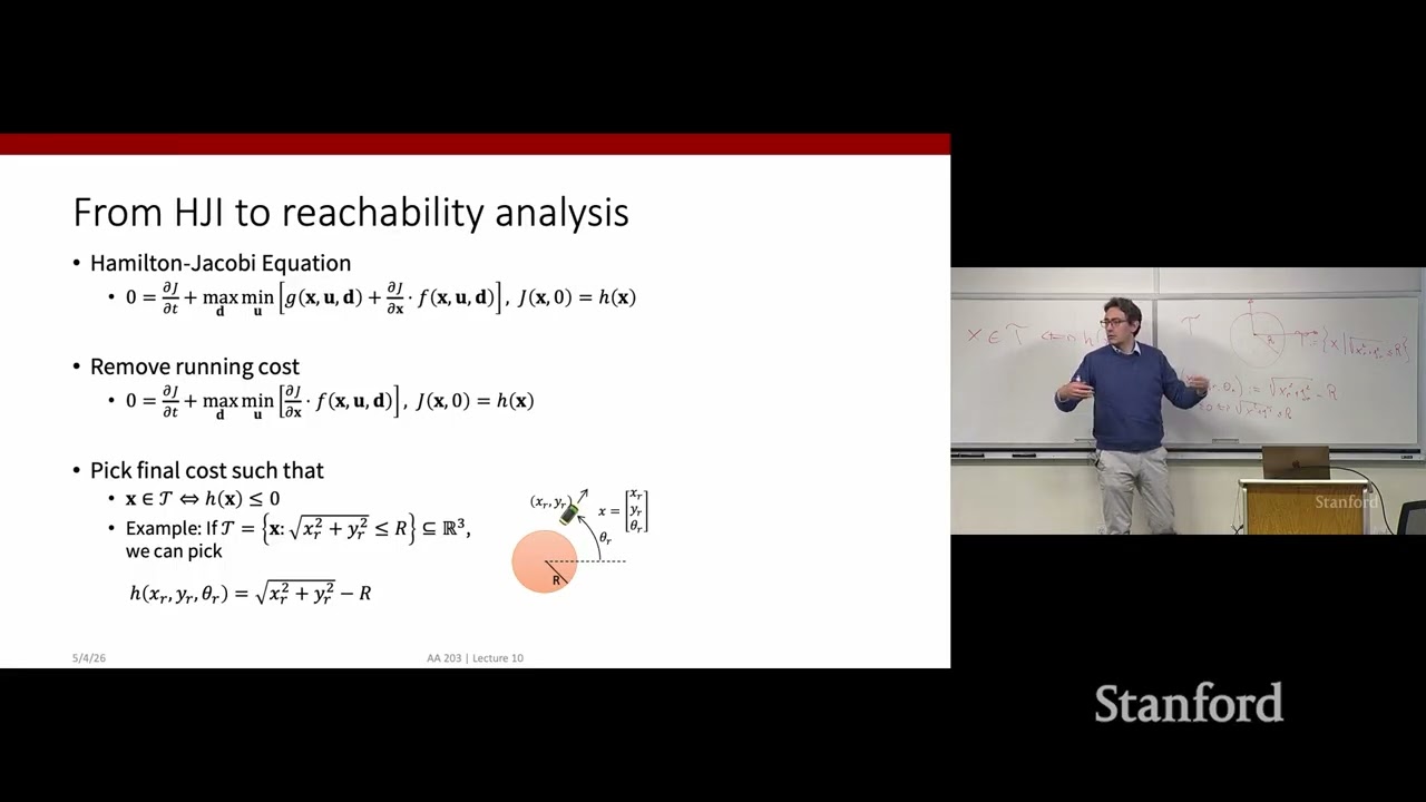
This lecture provides a deep dive into advanced control theory, transitioning from theoretical concepts like Hamilton-Jacobi-Isaacs (HJI) equations for computing reachable sets to the practical framework of Model Predictive Control (MPC). The discussion emphasizes that MPC achieves closed-loop performance by repeatedly solving an open-loop optimal control problem over a finite horizon (receding horizon optimization). Key theoretical challenges addressed include ensuring persistent feasibility and stability, which requires leveraging concepts from invariant set theory.
Key takeaways
-
Reachable Sets via HJI Equation
0:35
Avoidance sets and reachable sets are computed by solving a differential game using the Hamilton-Jacobi-Isaacs (HJI) equation. This involves reframing the Boolean problem of set membership into an optimal control cost function $h(x)$ [0:35].
-
Backward Reachable Tube (BRT)
7:40
To ensure safety over the entire trajectory, not just the endpoint, one must compute a Backward Reachable Tube (BRT). This is achieved by modifying the cost function to minimize the minimum value of $h(x)$ across the entire optimization horizon [7:40].
-
MPC Receding Horizon Principle
19:30
MPC solves an open-loop optimal control problem over a finite prediction horizon $[t, t+N_p]$ at each time step $t$. It then uses only the first computed input ($u_t$) and discards the rest of the plan, recomputing everything from scratch based on new state measurements (receding horizon) [19:30].
-
MPC Design Goals
36:00
The primary goals when designing an MPC controller are ensuring persistent feasibility (the problem remains solvable at all future times) and guaranteeing stability (convergence to the desired state, e.g., the origin) [36:00].
-
Invariant Sets for Feasibility
1:08:40
To guarantee persistent feasibility in MPC, one must identify a control invariant set $\mathcal{C}$. This is a set where, if the system starts within it, there exists a control input $u$ that guarantees the next state remains inside $\mathcal{C}$ [38:00].
Technical details
-
Hamilton-Jacobi-Isaacs (HJI) Equation
80s
Used to compute backward reachable sets. The problem is framed as a differential game between the controller (Player 1, minimizing cost) and nature/disturbance (Player 2, maximizing cost). Set membership $T$ is encoded by finding a function $h(x)$ such that $x ext{ belongs to } T ext{ if and only if } h(x) \le 0$ [0:50].
-
MPC Formulation (Linear Time-Invariant System)
1440s
The core problem is minimizing an additive cost subject to dynamics ($x_{t+1} = Ax_t + Bu$), state constraints $x \in \mathcal{X}$, and control constraints $u \in \mathcal{U}$. The formulation includes terminal cost and terminal constraints ($\mathcal{X}_f$) as tuning knobs [24:00].
-
Closed-Loop Policy Definition
1290s
The closed-loop policy is defined by the first control input $u_t$ computed when solving the optimal control problem starting from state $x_t$. This process of replanning at every time step closes the loop, bridging open-loop and closed-loop methods [21:30].
-
Computational Limitations
2580s
Solving these problems is computationally intensive. The HJI equation solvers are limited by the curse of dimensionality, typically failing beyond five or six state dimensions without resorting to approximations like neural networks or sampling-based methods [43:00].
Mentioned resources
Channel & topics
Watch on YouTube · Back to latest
This independent, AI-assisted summary is provided for commentary and informational purposes. It may contain errors or omit important context. Please watch the original video for the creator's complete presentation. Video, thumbnail, and related copyrights belong to their respective owners.