Topic

Policy Gradient

All digests tagged Policy Gradient

· 1:18:56

Stanford CS229 Machine Learning | Spring 2026 | Lecture 20: GMM (EM), PCA

This lecture provides an advanced deep dive into training Large Language Models (LLMs) using Reinforcement Learning (RL). It reviews Policy Gradient methods, detailing the mathematical derivations and limitations. The core focus shifts to Proximal Policy Optimization (PPO), a critical algorithm for stabilizing RL updates by utilizing importance sampling ratios and clipping mechanisms. Finally, the lecture applies these concepts to LLM generation, explaining how Chain-of-Thought (CoT) prompting can be formalized as an MDP problem solved via PPO/SISO.

Key takeaways

  1. Policy Gradient Theory 20:40

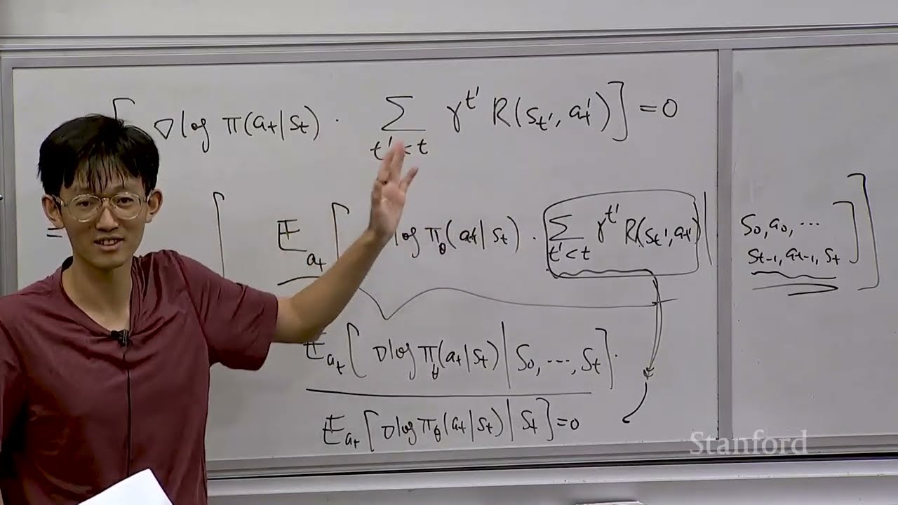
    The policy gradient estimator is necessary because the dependency on parameters ($ heta$) is complex. The fundamental property that $ abla_{ heta} ext{E}_{ ext{P}_{ heta}}[ abla_{ heta} ext{log } ext{P}_{ heta}(a|s)]$ equals zero shows that without a reward function, there are no preferences to optimize for.

  2. Proximal Policy Optimization (PPO) 26:40

    PPO is designed to stabilize RL training by using importance sampling and clipping the objective function. This prevents the new policy ($ heta$) from deviating too far from the old policy ($ heta_{old}$), which helps maintain stable learning.

  3. LLM Generation as an MDP 1:01:40

    The LLM generation process is modeled as a Markov Decision Process (MDP). The state ($s_t$) includes the history, and the action ($a_t$) is the next generated token. The reward function is typically applied only at the end of the trajectory based on whether the final answer matches the ground truth.

  4. Chain-of-Thought (CoT) Training 1:05:00

    To train models for complex reasoning, RL can be used to reward the entire trajectory based on the final answer's correctness. This approach bypasses the need for explicit labeling of the internal 'thinking tokens,' focusing only on verifiable outcomes.

Watch on YouTube Full article

· 1:16:25

Stanford CS229 Machine Learning | Spring 2026 | Lecture 18: GMM (EM), PCA

This lecture provides a deep dive into Reinforcement Learning (RL), focusing on the formal framework of Markov Decision Processes (MDPs) and the Policy Gradient method. The core objective is to solve sequential decision-making problems by maximizing expected cumulative reward. Key concepts include defining states ($S$), actions ($A$), stochastic transition dynamics ($P(s'|s, a)$), and utilizing the Bellman equation for recursive value estimation. The lecture concludes with an explanation of the Policy Gradient algorithm (REINFORCE), detailing how to compute the gradient of the expected return using log-probability tricks, which is crucial for training policies in large models.

Key takeaways

  1. Sequential Decision Making & RL Fundamentals

    RL addresses sequential decision-making where actions have long-term ramifications. It requires balancing the trade-off between exploitation (using current best knowledge) and exploration (gathering information). Learning relies on maximizing a scalar reward signal rather than explicit labels or supervision.

  2. Markov Decision Process (MDP) Framework 4:00

    An MDP formally describes an environment using five components: State Set ($S$), Action Set ($A$), Transition Dynamics ($P(s'|s, a)$), Reward Function ($R$), and Discount Factor ($\gamma$). The Markov property ensures that the future state transition depends only on the current state and action, not on history.

  3. Value Functions and Bellman Equation 28:50

    The value function $V^{\pi}(s)$ estimates the expected total payoff starting at state $s$ under policy $\pi$. The optimal value, $V^*(s)$, is the maximum possible return. These values are solved recursively using the Bellman equation, which relates the current state's value to the expected discounted future rewards.

  4. Policy Gradient Method (REINFORCE) 43:20

    The Policy Gradient algorithm optimizes a stochastic policy $\pi_{\theta}(a|s)$ by maximizing the expected return $E[R]$. The gradient is computed using the log-probability trick, allowing the calculation of $\nabla_{\theta} E[R]$ through sampling, even when the dependency on $\theta$ only affects the sampling distribution.

Watch on YouTube Full article